Additional material: Linear models and FDR
Last updated on 2025-11-19 | Edit this page
Estimated time 20 minutes
Overview
Questions
What are linear models?
What is a FDR?
Objectives
Explore linear models and learn how to interpret coefficients
Address the multiple testing issue
Parts of this chapter are based on the courses WSBIM1322 and Omics data analysis.
Multifactorial design and linear models
The outcome of an experiment, such as a gene expression level in the case of an RNA-seq, can be seen as the sum of several factors:
the treatments effects (these are the effects you actually want to study)
biological effects (representing natural biological differences between samples that you might also have to consider)
technical effects (that come from the experimental process itself and that could potentially influence the measurements)
and lastly, outcome will also reflect an error, which represent the random variability (or experiment noise) that cannot be explain be any of the known factors.
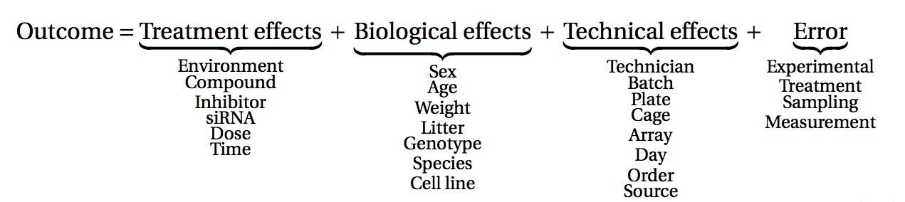
(figure from Lazic (2017)).
Single-factor design
Let’s start by a simple design, and let’s say we have the gene expression values of 3 control samples and 3 samples treated with a drug, assuming that there is no other biological effect or batch effect to consider.
We can use the following linear model to modelise the expression values:
\[y = \beta_0 + \beta_1 . x\]
In this equation,
\(y\) would be the measured expression level of a gene
the design factor \(x\) is a binary indicator variable representing the two groups of our experiment. It will take the value of 0 if we are considering the control samples, and a value of 1 when considering treated samples.
When considering a control sample, the \(x\) factor is set to 0.
The \(\beta_1 . x\) term is hence equal to 0, so the equation can be written:
\[y = \beta_0\]
This means that the \(\beta_0\) term represents the expression level of the gene in the control samples, this coefficient is usually called the intercept
When considering a treated sample, the \(x\) factor is set to 1.
The equation becomes:
\[y = \beta_0 + \beta_1\]
Assuming our expression values are in a log scale then
\[\beta_1 = y - \beta_0 = log(expression_{Treated\_cells}) - log(expression_{Control\_cells})\]
\[\beta_1 = log(\frac{expression_{Treated\_cells}}{expression_{Control\_cells}})\]
The \(\beta_1\) term represents hence the logFoldchange between the treated and the control samples (the treatment effect).
The goal is now to estimate the coefficients and test their significance
The \(\beta_0\) and \(\beta_1\) coefficients can be estimated from the data using the expression values in the control and in the treated samples.
A statistical test can then be applied, to test if the \(\beta_1\) coefficient (the logFC due to the treatment effect) is significantly different from 0.
The null hypothesis is that there is no difference across the sample groups, which is the same as saying that the \(\beta_1\) = 0.
- \(H_0\): \(\beta_1 = 0\) (the logFC = 0)
- \(H_1\): \(\beta_1 \neq 0\) (the logFC \(\neq\) 0)
Example
We are going to use as a toy example a subsetted version of the rna dataset. Let’s focus only on the first gene, the gene Asl, and let’s subset the table to keep only female mice at time 0 and 8.
R
rna <- read_csv("data/rnaseq.csv")
rna1 <- rna %>%
  filter(gene %in% c("Asl"), time %in% c(0,8), sex == "Female") %>%
  mutate(expression_log = log(expression)) %>%
  select(gene, sample, expression_log, time, infection, sex) %>%
  arrange(infection)
Let’s also convert the infection column into a factor,
in order to set the NonInfected condition as the reference
level.
R
rna1$infection <- factor(rna1$infection, levels = c("NonInfected", "InfluenzaA"))
Assuming the expression values follow a normal distribution (even
though, as we’ll see later, this isn’t actually true!) and let’s use the
lm() function to fit a linear model to compare infected
mice to non-infected mice.
In this case the design of our experiment would be :
\[design \sim infection\]
R
mod1 <- lm(expression_log ~ infection, data = rna1)
mod1
OUTPUT
Call:
lm(formula = expression_log ~ infection, data = rna1)

Coefficients:
        (Intercept)  infectionInfluenzaA
             6.0941               0.8358
The lm() function has estimated the coefficients of the linear model:
The estimate for the \(\beta_0\) coefficient (the
Intercept) is 6.0941The estimate for the \(\beta_1\) coefficient (annotated as the
infectionInfluenzaAcoefficient) is 0.8358
We can visualise this linear model with:
R
rna1 %>%
  ggplot(aes(x = infection, y = expression_log)) +
  geom_jitter() +
  geom_boxplot(alpha = 0) +
  geom_point(aes(x = "NonInfected", y = 6.094074), color = "blue", size = 4) +
  geom_point(aes(x = "InfluenzaA", y = 6.094074 + 0.8357904), color = "red", size = 4)
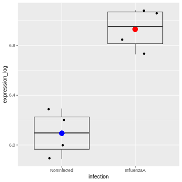
And indeed, we see that
– the intercept (the \(\beta_0\)
coefficient) corresponds to the mean expression level of the gene in the
Noninfected group corresponds (the blue dot)
– the sum of the \(\beta_0\) and the
\(\beta_1\) coefficients (the intercept
+ the logFC) corresponds to the mean expression level of the gene in the
InfluenzaA group (the red dot)
We can also extract the p-value associated with the
infectionInfluenzaA coefficient:
R
summary(mod1)
OUTPUT
Call:
lm(formula = expression_log ~ infection, data = rna1)

Residuals:
     Min       1Q   Median       3Q      Max
-0.20520 -0.12727  0.01064  0.13955  0.19934

Coefficients:
                    Estimate Std. Error t value Pr(>|t|)
(Intercept)          6.09407    0.08991  67.782 6.94e-10 ***
infectionInfluenzaA  0.83579    0.12715   6.573 0.000594 ***
---
Signif. codes:  0 '***' 0.001 '**' 0.01 '*' 0.05 '.' 0.1 ' ' 1

Residual standard error: 0.1798 on 6 degrees of freedom
Multiple R-squared:  0.8781,	Adjusted R-squared:  0.8578
F-statistic: 43.21 on 1 and 6 DF,  p-value: 0.0005944
We can see that the coefficient infectionInfluenzaA is
highly significant.
Two-factor design
Let’s consider a slightly more complex design. We now have the gene expression values of 6 control and 6 treated samples, but the experiment was conducted in 2 different cell types (cells A and cells B). We hence have 3 controls and 3 treated samples for each cell type.
To take into account the treatment effect while controlling the cell origin, we should use the following design: \[design \sim Treatment + Cell\]
in the following linear model:
\[y = \beta_0 + \beta_1 . x_1 + \beta_2 . x_2\]
We could rewrite this equation as:
\[y = \beta_0 + Treatment. x_1 + Cell . x_2\]
In this equation,
the \(\beta_0\) term represents the
intercept, i.e, the expression level of the gene in the reference sample, for instance the untreated cell type A.the design factor \(x_1\) is a binary indicator variable representing the two treatment conditions of our experiment. It will take the value of 0 if we are considering the untreated samples, and a value of 1 when considering treated samples.
The
Treatmentterm represents the logFoldchange due to treatment.the design factor \(x_2\) is another binary indicator variable representing the two cell types of our experiment. It will take the value of 0 if we are considering the cell type A, and a value of 1 when considering cell type B.
The
Cellterm represents the logFoldchange due to celltype.
The following figure (generated with the
ExploreModelMatrix package) illustrates the value of the
linear predictor of a linear model for each combination of input
variables.
OUTPUT
[[1]]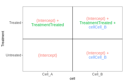
From this figure, we can see how the genes log expression values are modelised in the different samples:
In
untreated cells A: \(y\) = \(\beta_0\)In
treated cells A: \(y\) = \(\beta_0\) + TreatmentIn
untreated cells B: \(y\) = \(\beta_0\) + CellIn
treated cells B: \(y\) = \(\beta_0\) + Treatment + Cell
Example
Let’s subset the rna dataset as below to keep only on the gene Ddx3x, and mice at time 0 and 8.
R
rna2 <- rna %>%
  filter(gene %in% c("Ddx3x"), time %in% c(0,8)) %>%
  mutate(expression_log = log(expression)) %>%
  select(gene, sample, expression_log, time, infection, sex) %>%
  arrange(infection)

#set the `NonInfected` condition as the reference level.
rna2$infection <- factor(rna2$infection, levels = c("NonInfected", "InfluenzaA"))
We will start by fitting a linear model that only accounts for the infection effect, ignoring the sex effect.
Our design would hence be \[design \sim infection\]
R
mod2 <- lm(expression_log ~ infection, data = rna2)
summary(mod2)
OUTPUT
Call:
lm(formula = expression_log ~ infection, data = rna2)

Residuals:
     Min       1Q   Median       3Q      Max
-0.20156 -0.15940  0.02542  0.14115  0.19720

Coefficients:
                    Estimate Std. Error t value Pr(>|t|)
(Intercept)          9.94523    0.06150 161.710   <2e-16 ***
infectionInfluenzaA  0.15182    0.08697   1.746    0.106
---
Signif. codes:  0 '***' 0.001 '**' 0.01 '*' 0.05 '.' 0.1 ' ' 1

Residual standard error: 0.1627 on 12 degrees of freedom
Multiple R-squared:  0.2025,	Adjusted R-squared:  0.136
F-statistic: 3.047 on 1 and 12 DF,  p-value: 0.1064
The Infection Effect is not significant.
R
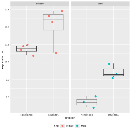
rna2 %>%
  ggplot(aes(x = infection, y = expression_log)) +
  geom_jitter(size = 3, aes(color = sex)) +
  geom_boxplot(alpha = 0) +
  theme(legend.position = "bottom")
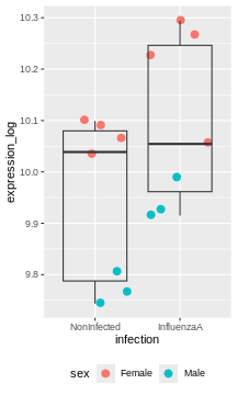
Challenge:
Try to figure our what is wrong with this model
The model only accounts for the infection effect. It ignores the sex effect.
Male and female values are mixed, even though they clearly don’t start at the same baseline.
Challenge:
Use the lm() function to fit a linear model that would
now account for infection and sex.
Interprete the results.
R
mod3 <- lm(expression_log ~ infection + sex, data = rna2)
summary(mod3)
OUTPUT
Call:
lm(formula = expression_log ~ infection + sex, data = rna2)

Residuals:
      Min        1Q    Median        3Q       Max
-0.163831 -0.019300  0.005398  0.030459  0.076010

Coefficients:
                    Estimate Std. Error t value Pr(>|t|)
(Intercept)         10.06641    0.02789 360.888  < 2e-16 ***
infectionInfluenzaA  0.15182    0.03364   4.513 0.000882 ***
sexMale             -0.28277    0.03399  -8.319 4.49e-06 ***
---
Signif. codes:  0 '***' 0.001 '**' 0.01 '*' 0.05 '.' 0.1 ' ' 1

Residual standard error: 0.06294 on 11 degrees of freedom
Multiple R-squared:  0.8906,	Adjusted R-squared:  0.8707
F-statistic: 44.79 on 2 and 11 DF,  p-value: 5.175e-06
The coefficients infectionInfluenzaA (representing the
Infection Effect) and the coefficient sexMale,
representing the Sex Effect, are both significant.
R
rna2 %>%
  ggplot(aes(x = infection, y = expression_log)) +
  geom_jitter(size = 3, aes(color = sex)) +
  geom_boxplot(alpha = 0) +
  facet_wrap(~ sex)+
  theme(legend.position = "bottom")
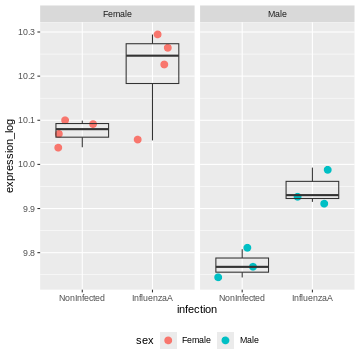
The model now adjusts for the baseline difference between males and females.
It prevents sex differences from biasing the infection effect.
Design with interaction
Coming back to the previous experimental design were we considered 3 controls and 3 treated samples for each cell type (cells A and cells B). An interaction term could be added to the linear model, to modelise a treatment effect that would differ across the cell types.
Our design would hence be : \[design \sim Treatment*Cell\]
The linear model could be written
\[y = \beta_0 + \beta_1 . x_1 + \beta_2 . x_2 + \beta_{12}.x_1.x_2.\]
We could rewrite this equation as:
\[y = \beta_0 + Treatment. x_1 + Cell . x_2 + Treatment.Cell.x_1.x_2\]
In this equation,
the \(\beta_0\) term represents the
intercept, i.e, the expression level of the gene in the reference sample, for instance the untreated cell type A.the design factor \(x_1\) will take the value of 0 if we are considering the untreated samples, and a value of 1 when considering treated samples.
The
Treatmentterm represents the treatment effect in the reference cell type. In this case it would represent the logFoldchange between treated and untreated celltype A.the design factor \(x_2\) will take the value of 0 if we are considering the cell type A, and a value of 1 when considering cell type B.
The
Cellterm represents the Celltype effect in the untreated cells. In this case it would represent the logFoldchange between untreated celltype A and untreated celltype A.The
Treatment.Cellterm represents the treatment effect that would be different in cell type B compared to cell type A. This term will only be considered in the equation when we are referring to treated celltype B (i.e. when \(x_1\) = 1 and \(x_2\) = 1)
The following figure (generated with the
ExploreModelMatrix package) illustrates the value of the
linear predictor of a linear model for each combination of input
variables.
OUTPUT
[[1]]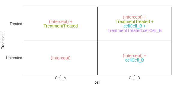
From this figure, we can see how the genes log expression values are modelised in the different samples:
In
untreated cells A: \(y\) = \(\beta_0\)In
treated cells A: \(y\) = \(\beta_0\) + TreatmentIn
untreated cells B: \(y\) = \(\beta_0\) + CellIn
treated cells B: \(y\) = \(\beta_0\) + Treatment + Cell + Treatment.Cell
Challenge:
Not let’s consider the exp dataset. Fit a linear model
with an interaction between condition and cell.
Interprete the results.
R
exp <- structure(list(
  gene = c("geneX", "geneX", "geneX", "geneX", "geneX", "geneX", "geneX",
           "geneX", "geneX", "geneX", "geneX", "geneX"),
  cell = c("cellA", "cellA", "cellA", "cellA", "cellA", "cellA", "cellB",
           "cellB", "cellB", "cellB", "cellB", "cellB"),
  condition = c("CTL", "CTL", "CTL", "treated", "treated", "treated",
                "CTL", "CTL", "CTL", "treated", "treated", "treated"),
  expression_log = c(10.3490970690873, 10.1575190636127, 10.4868623968153,
                     11.6188348660566, 12.7138479539555, 12.6343779570465,
                     10.0898526422682, 9.70416016607923, 10.4827957238796,
                     7.79590981240408, 8.18400846690037, 8.17157903656578)),
  class = c("tbl_df", "tbl", "data.frame"), row.names = c(NA, -12L))

exp
OUTPUT
# A tibble: 12 × 4
   gene  cell  condition expression_log
   <chr> <chr> <chr>              <dbl>
 1 geneX cellA CTL                10.3
 2 geneX cellA CTL                10.2
 3 geneX cellA CTL                10.5
 4 geneX cellA treated            11.6
 5 geneX cellA treated            12.7
 6 geneX cellA treated            12.6
 7 geneX cellB CTL                10.1
 8 geneX cellB CTL                 9.70
 9 geneX cellB CTL                10.5
10 geneX cellB treated             7.80
11 geneX cellB treated             8.18
12 geneX cellB treated 8.17R
mod4 <- lm(expression_log ~ condition * cell, data = exp)
summary(mod4)
OUTPUT
Call:
lm(formula = expression_log ~ condition * cell, data = exp)
Residuals:
Min 1Q Median 3Q Max
-0.70352 -0.19388 0.06951 0.19478 0.39149
Coefficients:
Estimate Std. Error t value Pr(>|t|)
(Intercept) 10.3312 0.2237 46.188 5.33e-11 ***
conditiontreated 1.9912 0.3163 6.295 0.000234 ***
cellcellB -0.2389 0.3163 -0.755 0.471771
conditiontreated:cellcellB -4.0330 0.4473 -9.015 1.83e-05 ***
---
Signif. codes: 0 '***' 0.001 '**' 0.01 '*' 0.05 '.' 0.1 ' ' 1
Residual standard error: 0.3874 on 8 degrees of freedom
Multiple R-squared: 0.9581, Adjusted R-squared: 0.9424
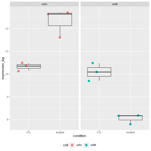
F-statistic: 60.99 on 3 and 8 DF, p-value: 7.452e-06The interaction term is significant. This indicates that the Treatement effect is significantly different in Cells A and cells B.
And indeed looking at the count values, we can see that the treatment increases the gene expression level in cells A, but it has an opposite effect in cells B.
Challenge:
Subset the rna dataset as below to keep only on the gene Ddx3x, and mice at time 0 and 8.
Re-use the previous rna2 dataset and fit a linear model
with an interaction between infection and sex.
Interprete the results.
R
mod3 <- lm(expression_log ~ infection * sex, data = rna2)
summary(mod3)
OUTPUT
Call:
lm(formula = expression_log ~ infection * sex, data = rna2)

Residuals:
      Min        1Q    Median        3Q       Max
-0.155912 -0.025986  0.005398  0.032198  0.083929

Coefficients:
                            Estimate Std. Error t value Pr(>|t|)
(Intercept)                 10.07433    0.03256 309.431  < 2e-16 ***
infectionInfluenzaA          0.13598    0.04604   2.953 0.014451 *
sexMale                     -0.30125    0.04973  -6.057 0.000122 ***
infectionInfluenzaA:sexMale  0.03696    0.07033   0.525 0.610714
---
Signif. codes:  0 '***' 0.001 '**' 0.01 '*' 0.05 '.' 0.1 ' ' 1

Residual standard error: 0.06512 on 10 degrees of freedom
Multiple R-squared:  0.8936,	Adjusted R-squared:  0.8616
F-statistic: 27.99 on 3 and 10 DF,  p-value: 3.529e-05
The coefficients infectionInfluenzaA (representing the
Infection Effect) and the coefficient sexMale,
representing the Sex Effect, are both significant.
But the interaction term is not. This indicates that the Infection Effect is not significantly different between males and females
This is not surprising because the effect is consistent in both sexes.
Multiple testing issue
In the few examples of linear model that we have seen in the previous
section, the lm() function was always applied to a single
gene. In a real RNA-seq experiment, we will have a few thousand tests to
perform, as each gene is going to be tested.
Let’s use the following dataset that provides log expression values for 20,000 genes in 6 samples, three in groupA and three in groupB.
R
if (!file.exists("data/exp.rda")) {
    dir.create("data", showWarnings = FALSE)
    download.file(
        url = "https://github.com/UCLouvain-BIOINFO/bioc-rnaseq/tree/main/episodes/data/exp.rda?raw=true",
        destfile = "data/exp.rda"
    )
}
load("data/exp.rda")
exp
OUTPUT
# A tibble: 20,000 × 7
   Gene      A1    A2    A3    B1    B2    B3
   <chr>  <dbl> <dbl> <dbl> <dbl> <dbl> <dbl>
 1 Gene1   4.72  4.89  4.51  4.00  4.66  4.67
 2 Gene2   4.61  4.96  4.58  4.53  4.21  4.78
 3 Gene3   4.75  4.70  4.75  4.55  4.89  4.31
 4 Gene4   4.83  4.83  4.43  4.53  4.38  4.55
 5 Gene5   4.68  4.33  4.84  4.58  4.64  4.92
 6 Gene6   4.57  4.74  4.68  4.84  4.42  4.96
 7 Gene7   4.68  4.47  4.50  4.55  4.23  4.67
 8 Gene8   4.59  4.81  4.44  4.45  4.20  4.61
 9 Gene9   4.53  4.84  4.51  4.53  4.61  4.59
10 Gene10  4.74  4.09  4.61  4.33  4.72  4.61
# ℹ 19,990 more rows
Let’s apply a t.test on all these genes
R
res <- exp %>%
  rowwise() %>%
  mutate(pval = t.test(c(A1, A2, A3), c(B1,B2,B3))$p.value) %>%
  ungroup() # to revert the rowwise()
res
OUTPUT
# A tibble: 20,000 × 8
   Gene      A1    A2    A3    B1    B2    B3  pval
   <chr>  <dbl> <dbl> <dbl> <dbl> <dbl> <dbl> <dbl>
 1 Gene1   4.72  4.89  4.51  4.00  4.66  4.67 0.367
 2 Gene2   4.61  4.96  4.58  4.53  4.21  4.78 0.362
 3 Gene3   4.75  4.70  4.75  4.55  4.89  4.31 0.474
 4 Gene4   4.83  4.83  4.43  4.53  4.38  4.55 0.249
 5 Gene5   4.68  4.33  4.84  4.58  4.64  4.92 0.632
 6 Gene6   4.57  4.74  4.68  4.84  4.42  4.96 0.679
 7 Gene7   4.68  4.47  4.50  4.55  4.23  4.67 0.682
 8 Gene8   4.59  4.81  4.44  4.45  4.20  4.61 0.286
 9 Gene9   4.53  4.84  4.51  4.53  4.61  4.59 0.689
10 Gene10  4.74  4.09  4.61  4.33  4.72  4.61 0.773
# ℹ 19,990 more rowsChallenge:
- How many significant genes did we obtained ? Which genes are of possible biological interest?
R
table(res$pval < 0.05)
OUTPUT
FALSE  TRUE
19324   676
R
res %>% filter(pval < 0.05) %>%
  arrange(pval)
OUTPUT
# A tibble: 676 × 8
   Gene         A1    A2    A3    B1    B2    B3      pval
   <chr>     <dbl> <dbl> <dbl> <dbl> <dbl> <dbl>     <dbl>
 1 Gene13793  4.41  4.38  4.42  4.75  4.74  4.73 0.0000613
 2 Gene35     4.47  4.45  4.42  4.79  4.75  4.79 0.000104
 3 Gene5006   4.79  4.78  4.75  4.56  4.59  4.57 0.000194
 4 Gene8102   4.31  4.30  4.35  4.60  4.67  4.64 0.000258
 5 Gene11686  4.58  4.60  4.61  4.77  4.74  4.75 0.000266
 6 Gene18641  4.35  4.42  4.35  4.78  4.70  4.78 0.000432
 7 Gene1936   4.47  4.54  4.49  4.79  4.86  4.86 0.000437
 8 Gene14972  4.07  4.15  4.20  4.67  4.55  4.68 0.000963
 9 Gene3211   4.74  4.81  4.75  4.38  4.30  4.42 0.00122
10 Gene10421  4.44  4.48  4.47  4.56  4.59  4.57 0.00153
# ℹ 666 more rows
The data above have been generated with the rnorm()
function for all samples.
This is the code that generated the data:
R
set.seed(2025)
exp <- matrix(rnorm(20000*6, mean = 100, sd = 20), ncol = 6)
rownames(exp) <- paste0("Gene", 1:20000)
colnames(exp) <- c(paste0("A", 1:3), paste0("B", 1:3))
exp <- log(exp)
exp <- as_tibble(exp, rownames = "Gene")
Challenge:
Do you still think any of the features show significant differences?
Why do we obtain genes with a p-value < 0.05?
A pvalue of 0.05 means that there is only 5% chance of getting this data if no real difference existed (if the null hypothesis was really true). In other words, choosing a cut off of 0.05 means there is 5% chance that the wrong decision is made (resulting in a false positive).
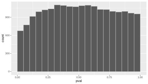
Challenge: Discuss
- If you were to visualize the p-value distribution using a histogram, how would you expect it to look like?
R
res %>%
  ggplot(aes(x = pval)) +
  geom_histogram(binwidth = 0.05, boundary = 0, color = "gray")
Now, let’s slightly modify our simulated expression data.
In a typical RNA-seq experiment, we may test around 20,000 genes, but only a fraction of them are expected to be truly differentially expressed. We could imagine a drug treatment that would modify the expression of about 1000 genes, but that would have no impact on the other ones.
To mimic this, we are going to simulate an up-regulation for the first 1,000 genes by increasing their expression values in group B.
R
exp_modified <- exp

exp_modified[1:1000, c("B1", "B2", "B3")] <- log(matrix(rnorm(1000*3, mean = 300, sd = 20), ncol = 3))

exp_modified <- exp_modified %>%
  mutate(DE = c(rep(TRUE, 1000), rep(FALSE, 19000)))

exp_modified
OUTPUT
# A tibble: 20,000 × 8
   Gene      A1    A2    A3    B1    B2    B3 DE
   <chr>  <dbl> <dbl> <dbl> <dbl> <dbl> <dbl> <lgl>
 1 Gene1   4.72  4.89  4.51  5.59  5.78  5.71 TRUE
 2 Gene2   4.61  4.96  4.58  5.73  5.76  5.73 TRUE
 3 Gene3   4.75  4.70  4.75  5.76  5.78  5.73 TRUE
 4 Gene4   4.83  4.83  4.43  5.64  5.66  5.75 TRUE
 5 Gene5   4.68  4.33  4.84  5.68  5.69  5.69 TRUE
 6 Gene6   4.57  4.74  4.68  5.63  5.79  5.84 TRUE
 7 Gene7   4.68  4.47  4.50  5.68  5.74  5.74 TRUE
 8 Gene8   4.59  4.81  4.44  5.78  5.68  5.74 TRUE
 9 Gene9   4.53  4.84  4.51  5.72  5.69  5.56 TRUE
10 Gene10  4.74  4.09  4.61  5.72  5.76  5.73 TRUE
# ℹ 19,990 more rows
Let’s run a t-test on this new dataset:
R
res_modified <- exp_modified %>%
  rowwise() %>%
  mutate(pval = t.test(c(A1, A2, A3), c(B1, B2, B3), var = TRUE)$p.value) %>%
  ungroup()
table(res_modified$pval < 0.05)
OUTPUT
FALSE  TRUE
18115 1885 Challenge: Discuss
How do think the histogram of the p-values of the first 1000 would look like?
What about the histogram of all p-values?
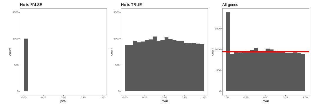
The figure on the right illustrates the principle behind the FDR adjustment. The False discovery rate (FDR) is the expected proportion of false positives among all the results considered as “significant” (i.e. pval < 0.05). The adjustment procedure estimate the proportion of hypothesis that are null and then adjust the p-values accordingly.
Adjustment for multiple testing
The False discovery rate (FDR) computes the expected fraction of false positives among all discoveries. It allows us to choose n results with a given FDR. Widely used examples are Benjamini-Hochberg or q-values.
let’s use the p.adjust() function to adjust the
pvalues.
R
res_modified <- res_modified %>%
  mutate(padj = p.adjust(pval, method = "BH"))

table(sign_padj = res_modified$padj < 0.05, sign_pval = res_modified$pval < 0.05)
OUTPUT
         sign_pval
sign_padj FALSE  TRUE
    FALSE 18115  1055
    TRUE      0   830
Only 830 were found to be significant after FDR correction.
Challenge:
- How many genes would you expect to remain significant after FDR correction in the first dataset?
R
res <- res %>%
  mutate(padj = p.adjust(pval, method = "BH"))
table(res$pval < 0.05)
OUTPUT
FALSE  TRUE
19324   676
R
table(res$padj < 0.05)
OUTPUT
FALSE
20000