Additional material: GSEA
Last updated on 2025-11-16 | Edit this page
Overview
Questions
- What is the aim of performing gene set enrichment analysis?
- What are the commonly-used gene set databases?
Objectives
- Learn how to obtain gene sets from various resources in R.
- Learn how to perform ORA and GSEA analyses
Objectives of an enrichment analysis
Once we have obtained a list of differentially expressed (DE) genes, the next question naturally to ask is what biological functions these DE genes may affect.
Gene set enrichment analyses (GSEA) evaluate the associations of a list of DE genes to a collection of pre-defined gene sets, where each gene set has a specific biological meaning. A geneset significantly enrichiched among DE genes could suggest that the corresponding biological process or pathway is significantly affected.
There are a huge amount of methods available for GSEA analysis. In this episode, we will focus on two widely used methods: the over-representation analysis (ORA) and the Gene set enrichment analysis (GSEA).
GeneSets
The definition of a gene set is very flexible and the construction of gene sets is straightforward. In most cases, gene sets are from public databases where huge efforts from scientific curators have already been made to carefully categorize genes into gene sets with clear biological meanings. For example, in a “cell cycle” gene set, all the genes are involved in the cell cycle process. Thus, if DE genes are significantly enriched in the “cell cycle” gene set, which means there are significantly more cell cycle genes differentially expressed than expected, we can conclude that the normal function of cell cycle process may be affected.
Nevertheless, gene sets can also be self-defined from individual studies, such as a set of genes in a network module from a co-expression network analysis, or a set of genes that are up-regulated in a certain disease.
The MSigDB database contains a collection of annotated gene sets such as
Gene Ontology (GO)
Gene Ontology defines concepts/classes used to describe gene function, and relationships between these concepts. GO terms are organized in a directed acyclic graph, where edges between terms represent parent-child relationship. It classifies functions along three aspects:
– MF: Molecular Function: molecular activities of gene
products
– CC: Cellular Component: where gene products are
active
– BP: Biological Process pathways and larger processes
made up of the activities of multiple gene products.
Hallmark gene setsare curated gene sets that represent well-defined biological states or processes (e.g. “Apoptosis”, “KRAS signaling”, “DNA repair”).Kyoto Encyclopedia of Genes and Genomes (KEGG)
KEGG is a collection of manually drawn pathway maps representing molecular interaction and reaction networks. These pathways cover a wide range of biochemical processes.
Other gene sets
Other gene sets include but are not limited to Positional gene sets, wikiPathways, Oncogenic signatures, Immunologic signatures…
Access the gene sets from MSigDB
The msigdbr CRAN package provides the MSigDB gene sets in a standard R data frame with key-value pairs.
One can use msigdbr_collections() to see the available collections
R
msigdbr_collections()
OUTPUT
# A tibble: 25 × 4
   gs_collection gs_subcollection  gs_collection_name               num_genesets
   <chr>         <chr>             <chr>                                   <int>
 1 C1            ""                Positional                                302
 2 C2            "CGP"             Chemical and Genetic Perturbati…         3538
 3 C2            "CP"              Canonical Pathways                         19
 4 C2            "CP:BIOCARTA"     BioCarta Pathways                         292
 5 C2            "CP:KEGG_LEGACY"  KEGG Legacy Pathways                      186
 6 C2            "CP:KEGG_MEDICUS" KEGG Medicus Pathways                     658
 7 C2            "CP:PID"          PID Pathways                              196
 8 C2            "CP:REACTOME"     Reactome Pathways                        1787
 9 C2            "CP:WIKIPATHWAYS" WikiPathways                              885
10 C3            "MIR:MIRDB"       miRDB                                    2377
# ℹ 15 more rows
R
GO_BP <- msigdbr(species = "Mus musculus", collection = "C5", subcollection = "BP") %>%
  dplyr::select(gs_name, gene_symbol)
OUTPUT
Using human MSigDB with ortholog mapping to mouse. Use `db_species = "MM"` for mouse-native gene sets.
This message is displayed once per session.Challenge:
How many genes belong to the
GOBP_REGULATION_OF_LYMPHOCYTE_MIGRATION geneset?
R
GO_BP %>%
  filter(gs_name == "GOBP_REGULATION_OF_LYMPHOCYTE_MIGRATION")
OUTPUT
# A tibble: 69 × 2
   gs_name                                 gene_symbol
   <chr>                                   <chr>
 1 GOBP_REGULATION_OF_LYMPHOCYTE_MIGRATION Abl1
 2 GOBP_REGULATION_OF_LYMPHOCYTE_MIGRATION Abl2
 3 GOBP_REGULATION_OF_LYMPHOCYTE_MIGRATION Adam10
 4 GOBP_REGULATION_OF_LYMPHOCYTE_MIGRATION Adam17
 5 GOBP_REGULATION_OF_LYMPHOCYTE_MIGRATION Adam8
 6 GOBP_REGULATION_OF_LYMPHOCYTE_MIGRATION Adtrp
 7 GOBP_REGULATION_OF_LYMPHOCYTE_MIGRATION Aif1
 8 GOBP_REGULATION_OF_LYMPHOCYTE_MIGRATION Aire
 9 GOBP_REGULATION_OF_LYMPHOCYTE_MIGRATION Akt1
10 GOBP_REGULATION_OF_LYMPHOCYTE_MIGRATION Apod
# ℹ 59 more rowsChallenge:
Retrieve Hallmarks genesets
R
hallmarks <- msigdbr(species = "Mus musculus", collection = "H") %>%
  dplyr::select(gs_name, gene_symbol)
Input data
We will use the differential expression analysis comparing infected mice at day8 and uninfected mice (day0). The following code performs DESeq2 analysis which you should have already learnt in the previous episode. We will focus on the genes that have an adjusted p-value (those that have been tested).
R
se <- readRDS("data/GSE96870_se.rds")
dds <- DESeqDataSet(se, design = ~ sex + time)
dds <- DESeq(dds)
res <- results(dds, name ="time_Day8_vs_Day0")
res_tbl <- as_tibble(res, rownames = "gene")

res_tbl <- res_tbl %>%
  filter(!is.na(padj))
ORA
Principle
The idea behind the ORA is to test whether your list of differentially expressed genes (DE) is enriched in certain biological categories (such as genesets from Gene Ontology terms, KEGG pathways, or Reactome pathways), i.e, if it contains more genes from these categories than would be expected by chance.
Step 1: selection of DE genes
To perform an over representation analysis, we first need to define the genes we will consider as differentially expressed (DE).
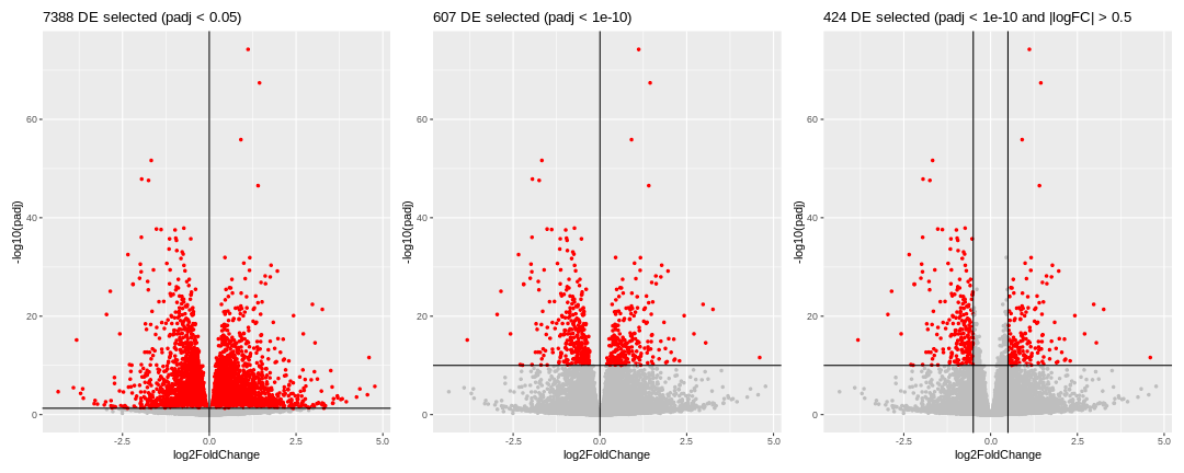
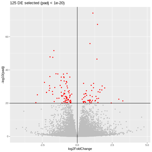
We could consider all genes that have a p-adjusted value < 0.05 (left volcano), in this case we would select 7388 genes. This number is probably too large, so we should probably be more restrictive and select a smaller set of genes, using a more stringent filtering on the p-adjusted value. We could also consider filtering using the logFC, which could also make biological sense.
Whatever thresholds are used, the idea here is to start from a selection of genes that we will consider as our DE genes. The selection is a choice the user has to make.
Here, we will apply the selection criteria illustrated in the third volcano. Hence, among all the genes (called the universe), we will consider the 424 genes with a p-adjusted value < 10^{-10} and an absolute logFoldChange > 0.5 as our genes of interest or DE genes.
Step2: Counting
For each biological category, we can count how many genes from our DE genes are in that category, and how many are not.
Let’s say we want to test the enrichment of the
GOBP_LEUKOCYTE_CHEMOTAXIS geneset.
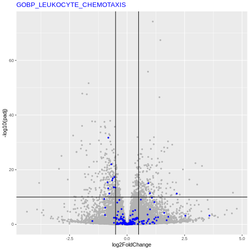
We will count the number of DE genes from that are in
GOBP_LEUKOCYTE_CHEMOTAXIS geneset, and how many are
not.
| GO | not_GO | |
|---|---|---|
| DE | 13 | 411 |
| not_DE | 180 | 23306 |
Step3: Statistical test
We can now apply a Fisher’s exact (or hypergeometric test) that will test whether there is a significant enrichment of DE genes in the GO term.
R
fisher.test(count_mat, alternative = "greater")
OUTPUT
	Fisher's Exact Test for Count Data

data:  count_mat
p-value = 4.378e-05
alternative hypothesis: true odds ratio is greater than 1
95 percent confidence interval:
 2.362979      Inf
sample estimates:
odds ratio
  4.094913
Running an ORA with clusterProfiler package
In practice, the analysis presented above can be executed using any of the very many packages that are available.
Here, we will use the clusterProfiler package to test if any GO terms from the Biological Process is enriched among our DE genes.
R
# Define our DE genes
padj_thr <- 1e-10
log2FC_thr <- 0.5
geneList <- res_tbl$gene
genes_DE <- res_tbl$gene[res_tbl$padj <= padj_thr &
                           abs(res_tbl$log2FoldChange) >= log2FC_thr]

ORA_res <- enricher(gene          = genes_DE,
                    universe      = geneList,
                    pAdjustMethod = "BH",
                    qvalueCutoff = 1,
                    pvalueCutoff = 1,
                    TERM2GENE     = GO_BP)

ORA_res_tbl <- as_tibble(ORA_res) %>% filter(p.adjust < 0.05)
ORA_res_tbl %>%
  select(ID, GeneRatio, BgRatio, pvalue, p.adjust)
OUTPUT
# A tibble: 6 × 5
  ID                                       GeneRatio BgRatio     pvalue p.adjust
  <chr>                                    <chr>     <chr>        <dbl>    <dbl>
1 GOBP_ENSHEATHMENT_OF_NEURONS             17/284    148/13271  1.76e-8  4.66e-5
2 GOBP_MYELIN_ASSEMBLY                     7/284     20/13271   1.17e-7  1.54e-4
3 GOBP_SECONDARY_ALCOHOL_METABOLIC_PROCESS 13/284    136/13271  6.92e-6  6.12e-3
4 GOBP_ALCOHOL_METABOLIC_PROCESS           19/284    294/13271  1.89e-5  1.25e-2
5 GOBP_STEROL_BIOSYNTHETIC_PROCESS         8/284     61/13271   4.39e-5  2.19e-2
6 GOBP_STEROID_METABOLIC_PROCESS           17/284    262/13271  4.96e-5  2.19e-2
In the output data frame, there are the following columns:
-
ID: ID of the gene set. In this example analysis, it is the GO ID. -
Description: Readable description. Here it is the name of the GO term. -
GeneRatio: Number of DE genes in the gene set / total number of DE genes. -
BgRatio: Size of the gene set / total number of genes. -
pvalue: p-value calculated from the hypergeometric distribution. -
p.adjust: Adjusted p-value by the BH method. -
qvalue: q-value which is another way for controlling false positives in multiple testings. -
geneID: A list of DE genes in the gene set. -
Count: Number of DE genes in the gene set.
You may have noticed the total number of DE genes changes. We defined 424 DE genes, but only 284 DE genes are included in the enrichment result table (in the GeneRatio column). Similarly, our universe had 23910 genes, but the total number of tested genes was only 13271 in the result table. The main reason is by default DE genes not annotated to any GO gene set are filtered out.
Visualisation
The clusterProfiler documentation provides a chapter on the visualization of functional enrichment results .
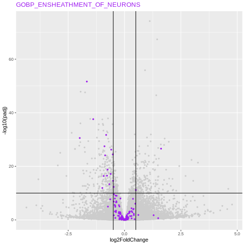
Another useful visualisation, that links the enrichment results back to the whole set of results is to highlight the genes in a particular set of interest on the volcano plot.
Let’s inspect genes from the GOBP_MYELINATIONon the
volcano
R
my_geneset <- "GOBP_ENSHEATHMENT_OF_NEURONS"
genes_from_geneset <- GO_BP %>%
  filter(gs_name == my_geneset) %>%
  pull(gene_symbol)

padj_thr <- 1e-10
log2FC_thr <- 0.5

res_tbl %>%
  ggplot(aes(x = log2FoldChange, y = -log10(padj))) +
  geom_point(color = "gray80", size = 1) +
  geom_point(data = res_tbl %>% filter(gene %in% genes_from_geneset), color = "purple", size = 1) +
  theme(legend.position = "none") +
  geom_hline(yintercept = -log10(padj_thr)) +
  geom_vline(xintercept = log2FC_thr) +
  geom_vline(xintercept = -log2FC_thr) +
  ggtitle(paste0(length(genes_DE2), " DE selected (padj < ", padj_thr, ")")) +
  ggtitle(my_geneset) +
  theme(title = element_text(color = "purple"),
        axis.title = element_text(color = "black"))
Conclusion about ORA method
This approach is straightfoward and very fast. Its major drawback however is that we need to define a cutoff to differentiate DE from non-DE genes. Setting this threshold might have an effect on the results.
Challenge:
Test a different threshold to define the group of ‘DE genes’ and check if, in the cases above, this has and effect on the GO terms of interest.
R
# Define our DE genes
padj_thr <- 1e-20
log2FC_thr <- 0

geneList <- res_tbl$gene
genes_DE <- res_tbl$gene[res_tbl$padj <= padj_thr &
                           abs(res_tbl$log2FoldChange) >= log2FC_thr]

res_tbl %>%
  ggplot(aes(x = log2FoldChange, y = -log10(padj))) +
  geom_point(aes(color = gene %in% genes_DE), size = 1) +
  scale_color_manual(values = c("gray", "red")) +
  theme(legend.position = "none") +
  geom_hline(yintercept = -log10(padj_thr)) +
  geom_vline(xintercept = log2FC_thr) +
  ggtitle(paste0(length(genes_DE), " DE selected (padj < ", padj_thr, ")"))
R
ORA_res_new_thr <- enricher(gene          = genes_DE,
                 universe      = geneList,
                 pAdjustMethod = "BH",
                 qvalueCutoff = 1,
                 pvalueCutoff = 1,
                 TERM2GENE     = GO_BP)

ORA_res_new_thr_tbl <- as_tibble(ORA_res_new_thr) %>% filter(p.adjust < 0.05)
ORA_res_new_thr_tbl %>%
  select(ID, GeneRatio, BgRatio, pvalue, p.adjust)
OUTPUT
# A tibble: 8 × 5
  ID                                          GeneRatio BgRatio  pvalue p.adjust
  <chr>                                       <chr>     <chr>     <dbl>    <dbl>
1 GOBP_ENSHEATHMENT_OF_NEURONS                9/102     148/13… 1.98e-6  0.00294
2 GOBP_NEURON_PROJECTION_REGENERATION         6/102     55/132… 3.80e-6  0.00294
3 GOBP_RESPONSE_TO_AXON_INJURY                6/102     76/132… 2.52e-5  0.0130
4 GOBP_REGENERATION                           8/102     162/13… 3.44e-5  0.0133
5 GOBP_ALCOHOL_METABOLIC_PROCESS              10/102    294/13… 8.62e-5  0.0267
6 GOBP_GLUTAMINE_FAMILY_AMINO_ACID_BIOSYNTHE… 3/102     14/132… 1.51e-4  0.0389
7 GOBP_ORGANIC_ACID_BIOSYNTHETIC_PROCESS      9/102     273/13… 2.49e-4  0.0492
8 GOBP_CELLULAR_COMPONENT_ASSEMBLY_INVOLVED_… 6/102     115/13… 2.54e-4  0.0492
R
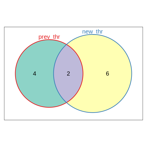
library(Vennerable)
geneset_list <- list(prev_thr = ORA_res_tbl$ID,
                     new_thr = ORA_res_new_thr_tbl$ID)
plot(Venn(geneset_list))
Challenge:
Repeat the ORA analysis using this time the Hallmarks genesets.
R
hallmarks <- msigdbr(species = "Mus musculus", collection = "H") %>%
  dplyr::select(gs_name, gene_symbol)

ORA_hallmarks <- enricher(gene          = genes_DE,
                          universe      = geneList,
                          pAdjustMethod = "BH",
                          qvalueCutoff = 1,
                          pvalueCutoff = 1,
                          TERM2GENE     = hallmarks)

ORA_hallmarks_tbl <- as_tibble(ORA_hallmarks) #%>% filter(p.adjust < 0.05)
ORA_hallmarks_tbl %>%
  select(ID, GeneRatio, BgRatio, pvalue, p.adjust)
OUTPUT
# A tibble: 31 × 5
   ID                               GeneRatio BgRatio  pvalue p.adjust
   <chr>                            <chr>     <chr>     <dbl>    <dbl>
 1 HALLMARK_XENOBIOTIC_METABOLISM   4/35      185/4049 0.0733    0.830
 2 HALLMARK_FATTY_ACID_METABOLISM   3/35      148/4049 0.134     0.830
 3 HALLMARK_PEROXISOME              2/35      95/4049  0.198     0.830
 4 HALLMARK_ANDROGEN_RESPONSE       2/35      99/4049  0.210     0.830
 5 HALLMARK_BILE_ACID_METABOLISM    2/35      101/4049 0.217     0.830
 6 HALLMARK_IL2_STAT5_SIGNALING     3/35      187/4049 0.218     0.830
 7 HALLMARK_TNFA_SIGNALING_VIA_NFKB 3/35      187/4049 0.218     0.830
 8 HALLMARK_MTORC1_SIGNALING        3/35      196/4049 0.239     0.830
 9 HALLMARK_APICAL_SURFACE          1/35      42/4049  0.307     0.830
10 HALLMARK_KRAS_SIGNALING_DN       2/35      153/4049 0.384     0.830
# ℹ 21 more rows
GSEA
Principle
Gene set enrichment analysis refers to a broad family of tests. Here, we will define the principles based on Subramanian et al. 2005 keeping in mind that the exact implementation will differ in different tools.
Gene Set Enrichment Analysis (GSEA) is a statistical method used to determine whether predefined sets of genes (for example, genes belonging to a GO term) show systematic differences in expression between two biological conditions. Instead of focusing only on individual genes, GSEA evaluates the collective behavior of gene groups.
The major advantage of GSEA approaches is that they don’t rely on defining DE genes.
Step 1: Gene ranking
The first step is to order the genes of interest. Genes could be ranked for example by the value of the test statistic or by their p-value.
Depending on the metric used for the ranking, genes will be ordered from the most up-regulated to the most down-regulated (if the test statistic is used for instance) or by the most significantly DE (no matter if they are up or down-regulated) to genes not differentially expressed.
Step 2: Check where the genes of a specific geneset appear
For a given gene set (a GO-term for example), The idea is to check if these genes tend to appear toward the top or bottom of the ranked list, rather than being randomly scattered.
Step 3: Compute an Enrichment Score (ES)
The algorithm walks down the ranked list, increasing a running-sum statistic when it encounters a gene from the set, and decreasing it otherwise.
The positive score is defined by \(\frac{n_{genes} - n_{genes~in~set}}{n_{genes~in~set}}\), and the decreasing score by -1, so that the sum of all genes in the set and those not in the set becomes zero.
The maximum deviation from zero is the Enrichment Score (ES), reflecting how strongly the gene set is enriched at either end of the ranking.
Step 4: Assess significance by permutation
To evaluate whether the observed ES is greater than expected by chance, GSEA performs permutations (of either gene labels or sample labels). This generates a null distribution to compute a p-value.
An Enrichment score is recomputed for each permutation. The p-value is given by the proportion of permutations where the permuted ES is at least as extreme as the observed ES:
\[p = \frac{\#\{ ES_{\text{permuted}} \ge ES_{\text{observed}} \}}{\text{total number of permutations}}\]
Running a GSEA with clusterProfiler package
Here, we will re-use the clusterProfiler package to run a GSEA this time, using GO terms from the Biological Process.
R
# Ranking our DE results by the statistic value used in DESeq2
geneList <- res_tbl$stat
names(geneList)<- res_tbl$gene
geneList <- geneList[order(geneList, decreasing = TRUE)]

set.seed(1)
GSEA_res <- GSEA(geneList,
             seed = TRUE,
             TERM2GENE = GO_BP,
             verbose = FALSE,
             by = "fgsea",
             pvalueCutoff = 1,
             pAdjustMethod = "BH",
             eps = 0)
GSEA_res_tbl <- as_tibble(GSEA_res) %>% filter(p.adjust < 0.05)
GSEA_res_tbl %>% select(ID, setSize, enrichmentScore, NES, pvalue, p.adjust)
OUTPUT
# A tibble: 92 × 6
ID setSize enrichmentScore NES pvalue p.adjust
<chr> <int> <dbl> <dbl> <dbl> <dbl>
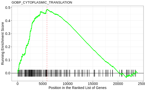
1 GOBP_CYTOPLASMIC_TRANSLATION 164 0.487 2.12 1.16e-9 3.87e-6
2 GOBP_PROTEIN_FOLDING 200 -0.470 -2.05 1.55e-9 3.87e-6
3 GOBP_AXON_DEVELOPMENT 499 -0.363 -1.73 1.99e-8 3.31e-5
4 GOBP_SUBSTANTIA_NIGRA_DEVELOP… 43 -0.694 -2.34 2.81e-8 3.51e-5
5 GOBP_ENSHEATHMENT_OF_NEURONS 148 -0.490 -2.05 4.72e-8 4.71e-5
6 GOBP_NEURAL_NUCLEUS_DEVELOPME… 63 -0.614 -2.24 2.41e-7 2.01e-4
7 GOBP_MIDBRAIN_DEVELOPMENT 87 -0.545 -2.10 6.88e-7 4.91e-4
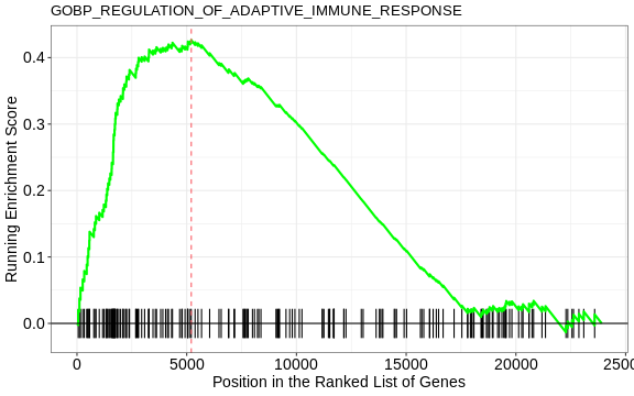
8 GOBP_REGULATION_OF_ADAPTIVE_I… 183 0.426 1.89 9.67e-7 5.62e-4
9 GOBP_REGULATION_OF_LEUKOCYTE_… 205 0.409 1.84 1.01e-6 5.62e-4
10 GOBP_REGULATION_OF_LYMPHOCYTE… 149 0.454 1.95 1.37e-6 6.87e-4
# ℹ 82 more rowsIn the output data frame, there are the following columns:
-
ID: ID of the gene set. In this example analysis, it is the GO ID. -
Description: Readable description. Here it is the name of the GO term. -
setSize: Number of genes in this gene set that are present in your universe of tested genes. -
enrichmentScore: Raw enrichment score calculated from the running-sum statistic. -
NES: ES normalized by gene set size. T -
pvalue: p-value calculated from the hypergeometric distribution. -
p.adjust: Adjusted p-value by the BH method. -
qvalue: q-value which is another way for controlling false positives in multiple testings. -
rank: Position in the ranked gene list where the running score reaches its maximum (the ES). -
leadingEdge: List of genes in the set contributing most to the ES (genes before the peak), often called the core enrichment.
The GSEA plot can be drawn with the gseaplot() function
R
gseaplot(GSEA_res, GSEA_res_tbl$ID[1], by = "runningScore", title = GSEA_res_tbl$ID[1])
Challenge:
Think about the different ways to order the genes for the GSEA analysis. What impact could the ranking method have on the GSEA analysis?
Compare GSEA and ORA methods, what are pros and cons of both methods?
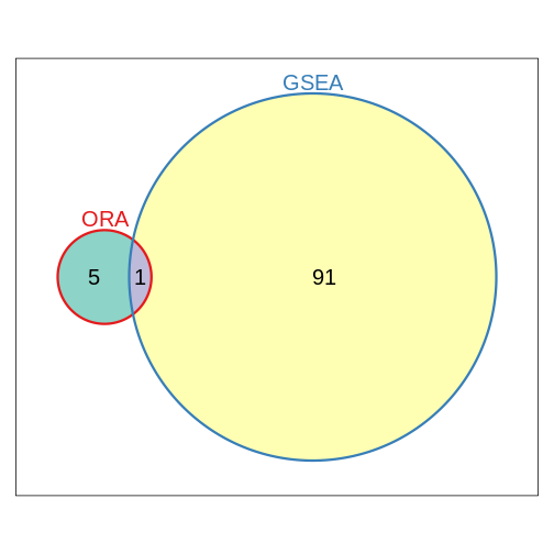
Compare the results obtained using ORA and GSEA on GO terms (BP)
R
library(Vennerable)
geneset_list <- list(ORA = ORA_res_tbl$ID,
                     GSEA = GSEA_res_tbl$ID)
plot(Venn(geneset_list))